Off the Planckian Locus: Using 2D Chromaticity to Improve In-Camera Color

Angular color reproduction error for a ColorChecker chart under illuminants on and off the Planckian locus, comparing 1D interpolation with our 2D prediction — **1D Planckian interpolation vs. our 2D chromaticity-based prediction.** Traditional 1D methods perform adequately for light sources whose CCTs lie close to the Planckian locus, but are less accurate for sources, namely LEDs, that lie off it. Heat maps show angular reproduction error, from 0° (dark blue) to 15° (dark red).

Abstract

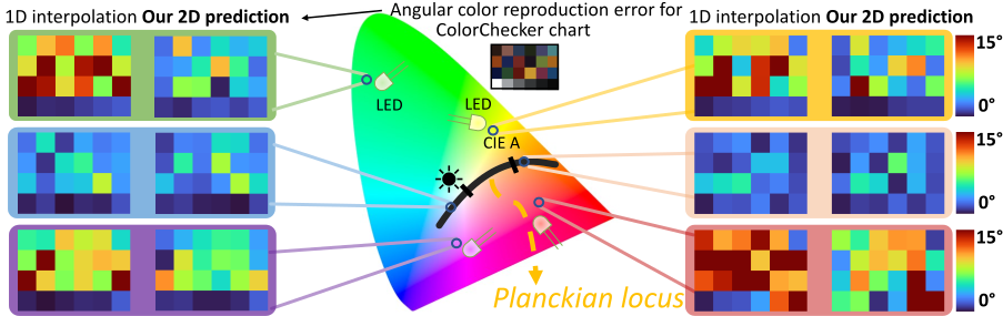
Traditional in-camera colorimetric mapping relies on correlated color temperature (CCT)-based interpolation between pre-calibrated transforms optimized for Planckian illuminants such as CIE A and D65. However, modern lighting technologies such as LEDs can deviate substantially from the Planckian locus, exposing the limitations of relying on conventional one-dimensional CCT for illumination characterization. This paper demonstrates that transitioning from 1D CCT (on the Planckian locus) to a 2D chromaticity space (off the Planckian locus) improves colorimetric accuracy across various mapping approaches. In addition, we replace conventional CCT interpolation with a lightweight multi-layer perceptron (MLP) that leverages 2D chromaticity features for robust colorimetric mapping under non-Planckian illuminants. A lightbox-based calibration procedure incorporating representative LED sources is used to train our MLP. Validated across diverse LED lighting, our method reduces angular reproduction error by 22% on average in LED-lit scenes, maintains backward compatibility with traditional illuminants, accommodates multi-illuminant scenes, and supports real-time in-camera deployment with negligible additional computational cost.

Video

1D CCT vs. 2D Chromaticity

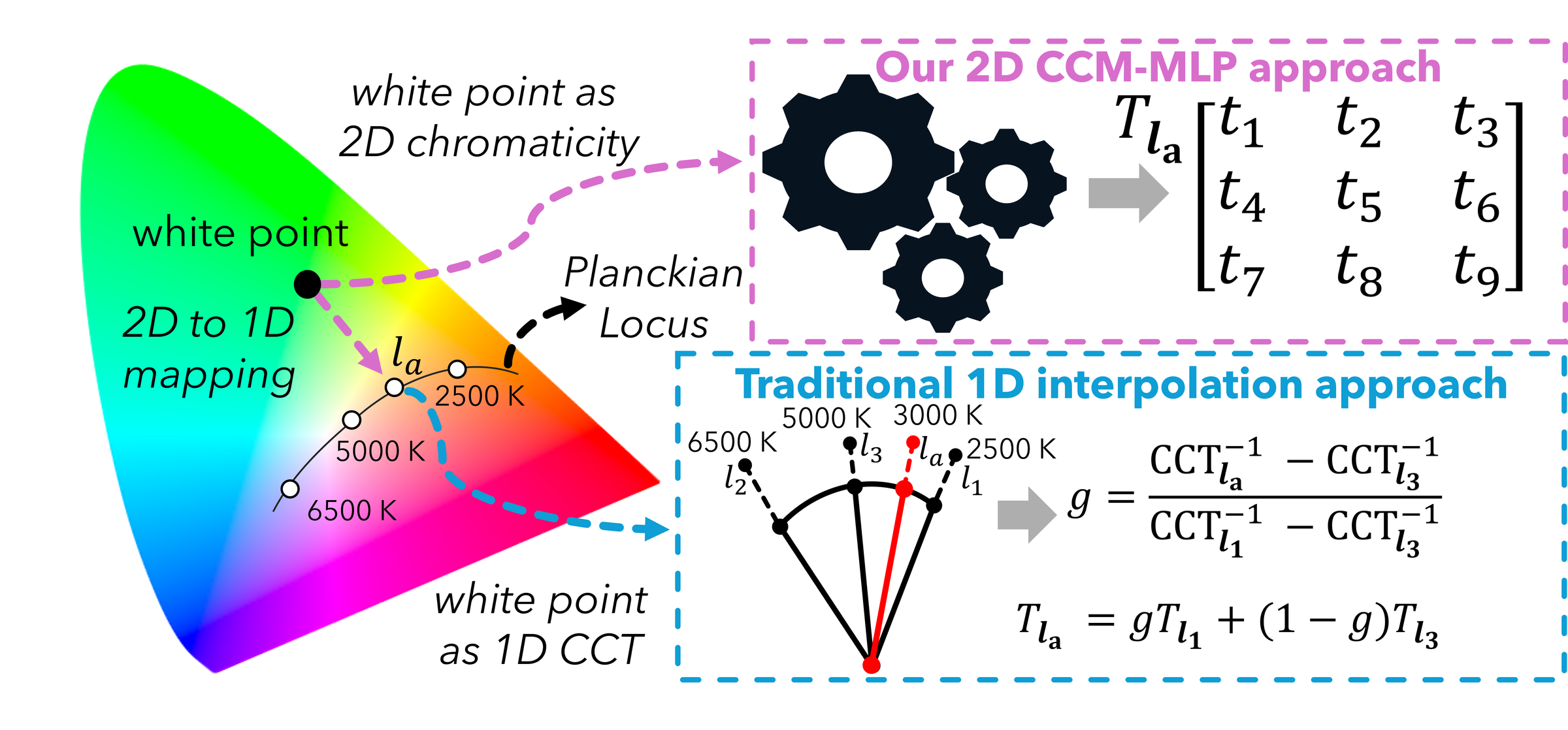
The standard procedure computes the color correction matrix by interpolating pre-calibrated matrices along the Planckian locus, characterizing the light with a single number: its correlated color temperature. Modern LEDs, however, exhibit chromaticities that deviate significantly from that locus, where a CCT no longer describes them adequately. We therefore shift from a one-dimensional CCT space to a 2D chromaticity space, and predict the matrix directly.

Our 2D chromaticity CCM-MLP approach compared with traditional 1D Planckian interpolation — **2D chromaticity CCM prediction vs. 1D CCT interpolation.** Interpolation approaches assume the CCM can be derived from illuminants calibrated along the Planckian locus. Our CCM-MLP instead predicts the full 3×3 matrix from 2D chromaticity coordinates.

In-Camera Pipeline

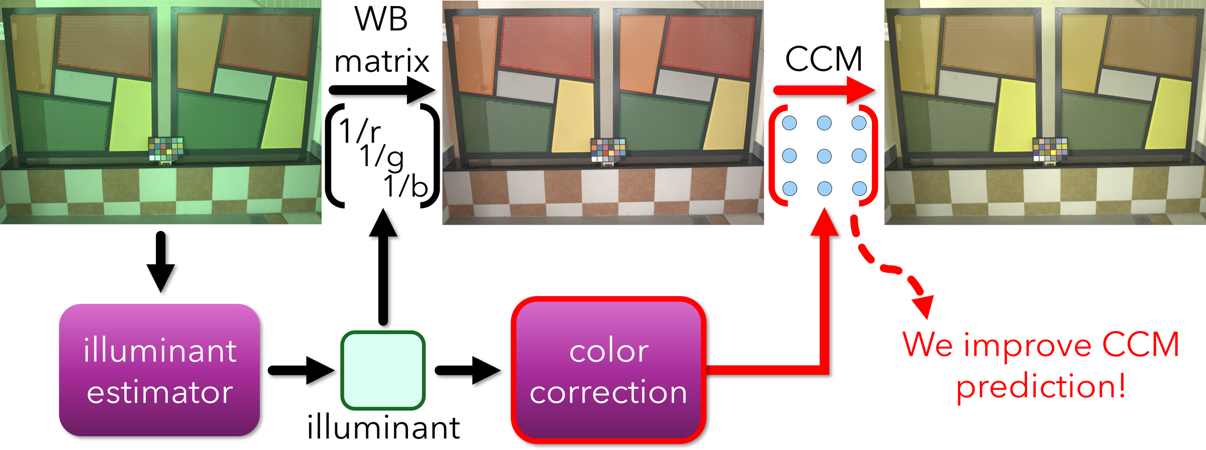
Digital cameras apply a long chain of processing routines to convert sensor-specific RGB responses into a final output image. Among these, the colorimetric mapping stage maps sensor values into a standard color space such as CIE XYZ, and its accuracy determines color reproduction quality across lighting conditions.

Colorimetric Mapping Stage

The estimated illuminant corrects neutral colors through a diagonal white balance matrix, but non-neutral colors require a further, illumination-specific 3×3 color correction matrix (CCM) that maps white-balanced raw-RGB into CIE XYZ. It is this matrix that we predict, as a drop-in replacement for the existing stage.

Method

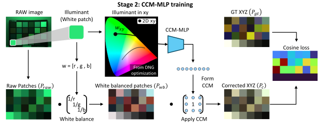
We learn a mapping from illuminant chromaticity to a CCM. CCM-MLP is a ReLU MLP with a single hidden layer of 32 neurons and eight outputs, which are reshaped into the 3×3 matrix; it takes the illuminant's xy chromaticity as input and is trained with a cosine loss against the ground-truth XYZ patches. The resulting model occupies 1.5 KB.

CCM-MLP training: raw image and white patch to illuminant chromaticity, MLP predicts CCM, cosine loss against ground truth XYZ patches — **CCM-MLP training.** Raw color patches are white balanced using the estimated illuminant, whose chromaticity is then fed to the MLP to predict the CCM. Training minimizes a cosine loss between the corrected and ground-truth XYZ patches.

Multi-illuminant extension

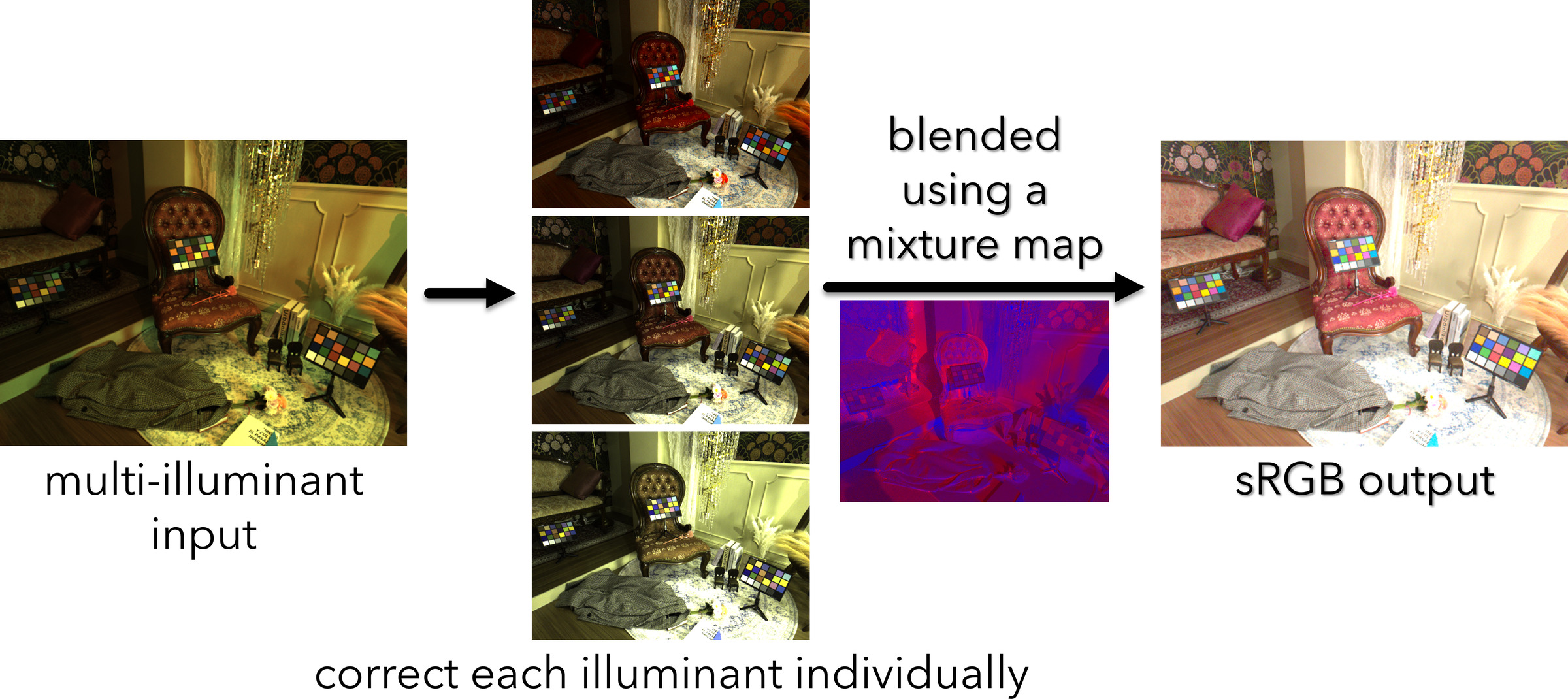
Assuming access to per-pixel illuminant information and a blending map, we predict and apply a CCM for each illuminant to produce several corrected versions of the white-balanced image, then merge them using the blending map as weights.

Multi-illuminant input, corrected once per illuminant, blended with a mixture map into the final sRGB output — **Multi-illuminant extension.** The input is corrected once per illuminant, and the results are blended with a mixture map to produce the sRGB output.

Dataset

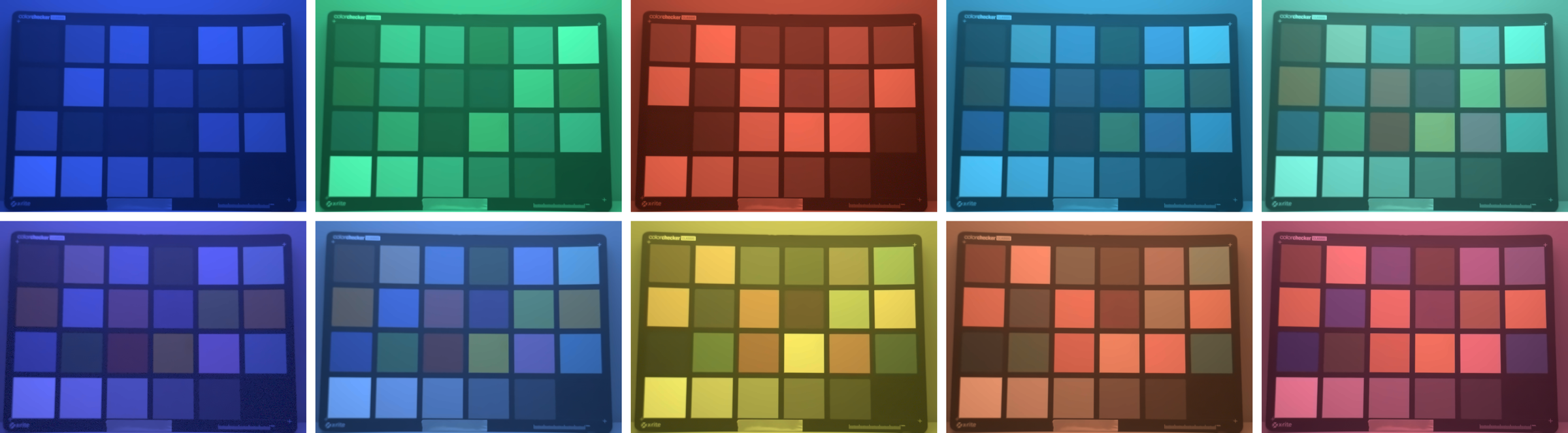
We capture a ColorChecker target under 790 illuminant spectra in a modified GTI lightbox fitted with tunable Telelumen LEDs, using two smartphones and two DSLRs. The illuminants cover the chromaticity space well beyond the Planckian locus, and are split into 395 training, 158 validation, and 237 test conditions.

A ColorChecker chart photographed under ten different LED illuminants, showing strong and varied color casts — **Lightbox captures.** The same ColorChecker target under ten of the 790 illuminants, many of which lie well off the Planckian locus.

In-the-wild scenes

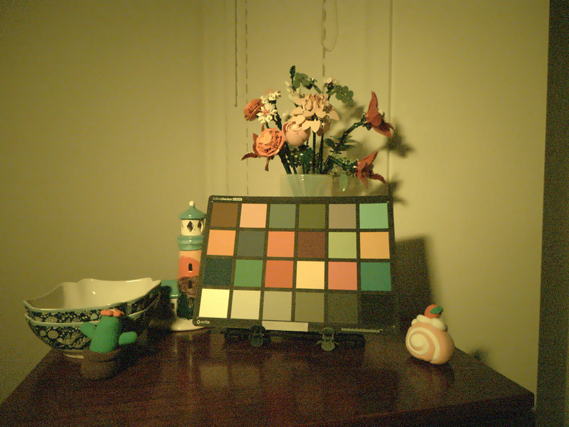
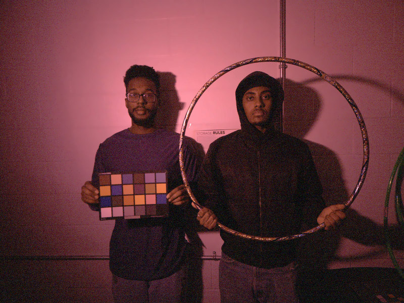
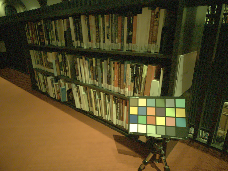
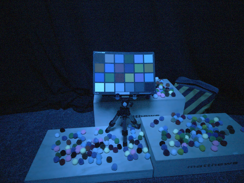
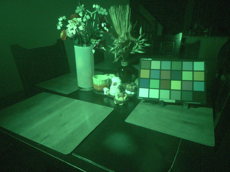
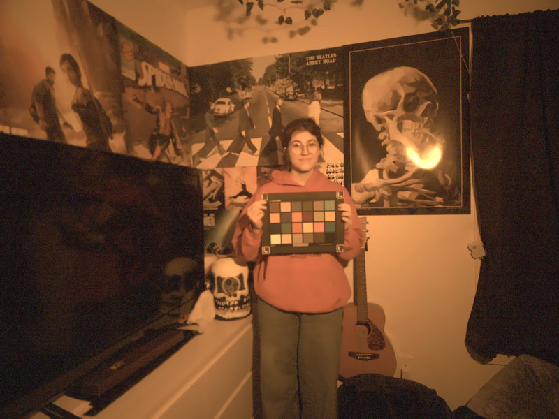
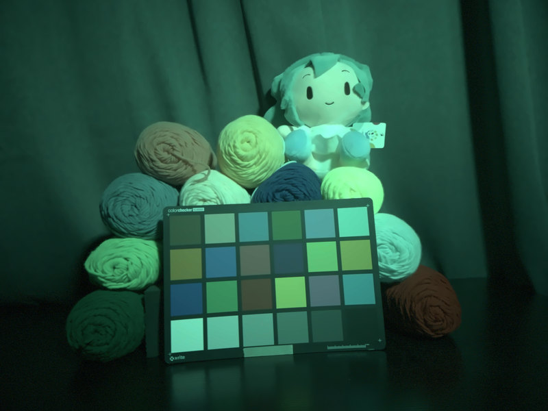
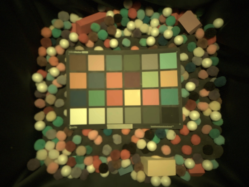
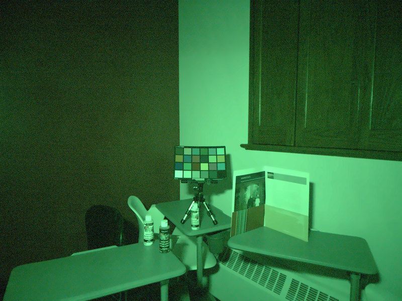
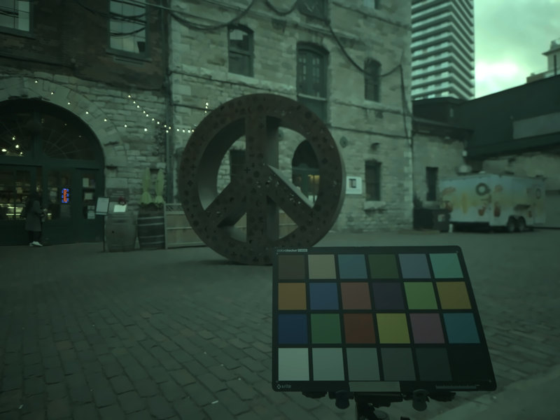
We further evaluate on 150 photographs taken with both smartphones under challenging LED illumination, covering skin tones, posters, and craft materials.

flowers and ceramics under warm LED — **In-the-wild dataset.** Real scenes under colored LED lighting, each captured with a ColorChecker present for ground truth.

two people holding a ColorChecker under magenta LED — **In-the-wild dataset.** Real scenes under colored LED lighting, each captured with a ColorChecker present for ground truth.

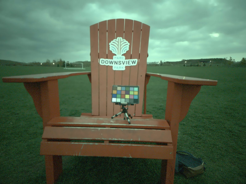
Quantitative Results

Rows using 2D chromaticity are shaded and the best result in each column is bold; Oracle denotes the upper bound given the full color chart rather than a competing method, and RP the root- polynomial variant. We find that all methods benefit from a 2D chromaticity coordinate over a 1D CCT.

Method	Dim	Size (KB)	MACs (M)	Angular error (°) ↓
Method	Dim	Size (KB)	MACs (M)	Mean	25%	50%	90%
Oracle	1D	0.00	0.01	2.79	0.95	2.00	5.94
2-CCM	1D	0.07	0.01	4.56	1.48	3.25	9.94
NN	1D	15.43	0.01	5.24	1.54	3.56	11.73
EXPINV	1D	68.53	13.39	4.31	1.26	2.85	9.88
CCM-MLP	1D	1.41	0.01	4.11	1.37	2.62	9.55
NN	2D	16.97	0.01	4.30	1.37	2.84	9.81
EXPINV	2D	69.03	13.48	3.84	1.32	2.71	8.41
CCM-MLP	2D	1.54	0.01	3.60	1.22	2.38	8.18
CCM-MLP (RP)	2D	2.70	0.01	3.27	1.13	2.14	7.47

Method	Dim	Angular error (°) ↓
Method	Dim	Single-illum.	Multi-illum.
Oracle	1D	2.38	2.06
2-CCM	1D	5.00	3.88
NN	1D	4.46	3.23
CCM-MLP	1D	3.77	2.52
CCM-MLP (RP)	1D	3.60	2.35
NN	2D	3.98	2.83
CCM-MLP	2D	3.49	2.26
CCM-MLP (RP)	2D	3.37	2.14

Full per-camera tables (Sony, Canon, Pixel, Samsung), ΔE₂₀₀₀, the NUS dataset, and the white-point sensitivity study are in the paper.

Qualitative Results

Colorimetric mapping results on the laboratory dataset for green and blue LED illuminants, Canon and Pixel cameras — **Lightbox dataset.** Results for two non-Planckian sources, a green LED (top half) and a blue LED (bottom half), captured with Canon and Pixel. Methods, left to right: 3-CCM, 1D EXPINV, 1D CCM-MLP, 2D EXPINV, 2D CCM-MLP, and ground truth.

Colorimetric mapping results on in-the-wild captures for green and orange LED illuminants, Pixel and Samsung cameras — **In-the-wild captures.** Green (top half) and orange (bottom half) LED illuminants captured with Pixel and Samsung. Note the color casts introduced by EXPINV, a per-pixel method, when applied to full-size images.

Colorimetric mapping results on multi-illuminant scenes from the LSMI dataset, Galaxy camera — **Multi-illuminant scenes (LSMI).** Two multi-illuminant scenes from the Galaxy camera, with angular errors shown at the bottom left of each color chart. Methods, left to right: 2-CCM, 1D NN, 1D CCM-MLP, 2D NN, 2D CCM-MLP, and Oracle.

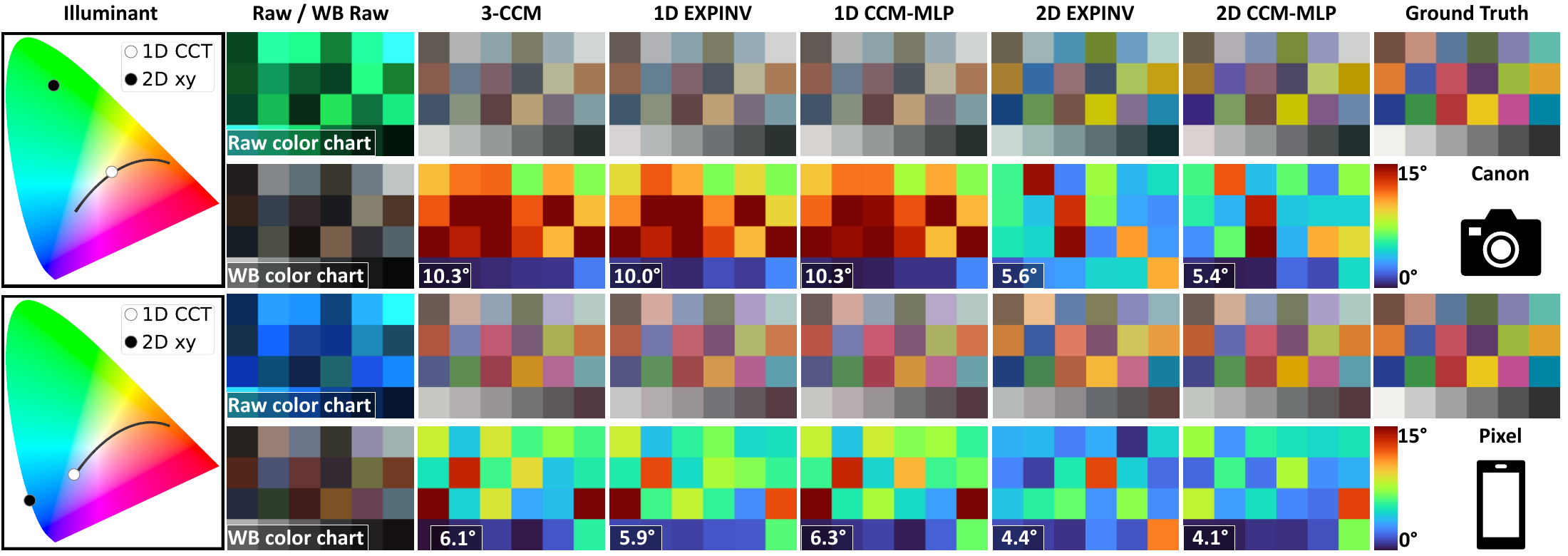
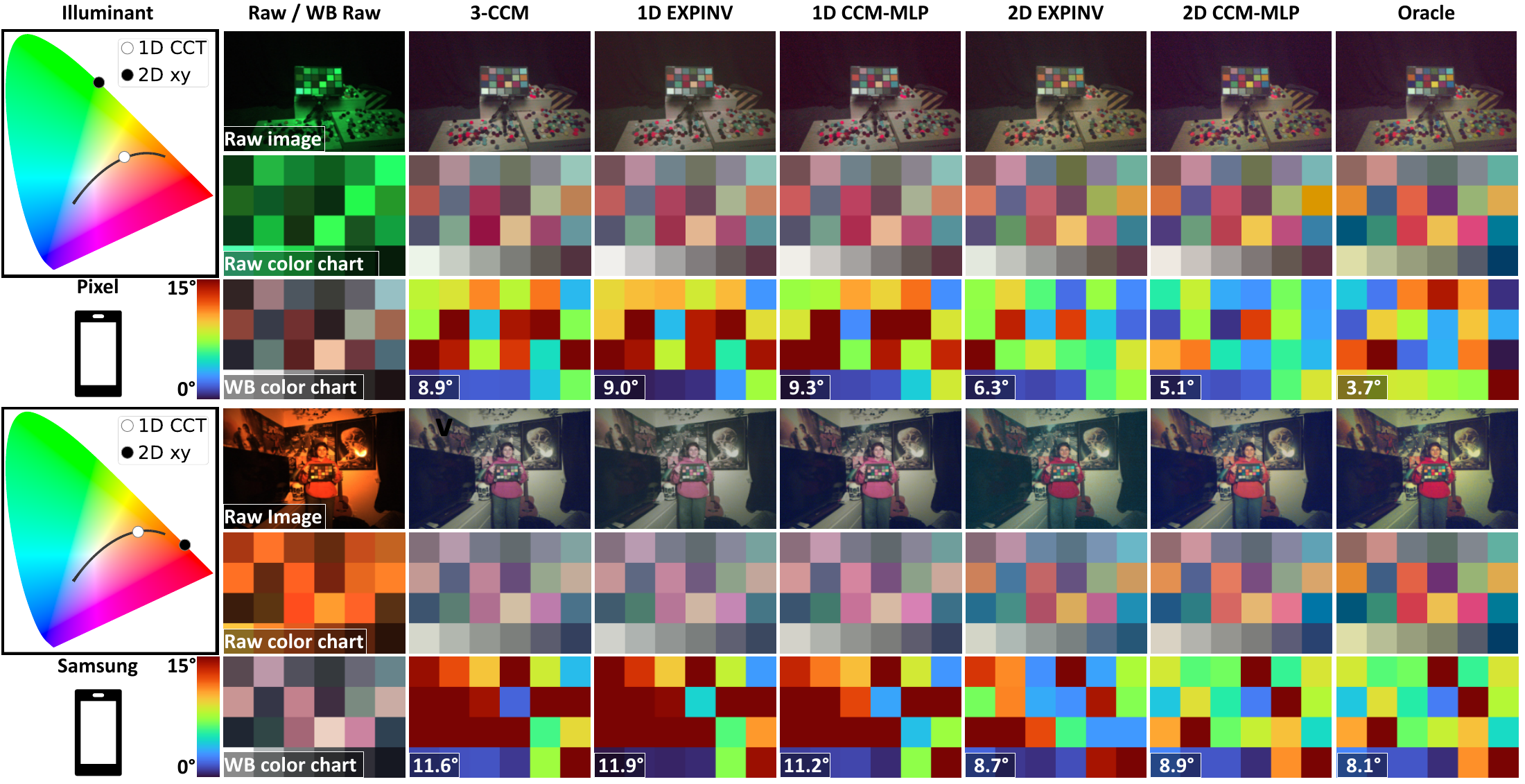
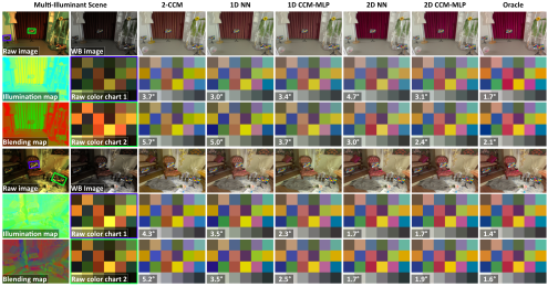
Computational Cost

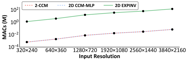
Because the CCM is computed once and applied to the entire image, CCM-MLP requires only 1.5 KB and 0.01 MMACs, compared with 69 KB and 13 MMACs for methods that must evaluate an MLP at every pixel.

Multiply-accumulate operations versus input resolution, log scale, for 2-CCM, our 2D CCM-MLP, and 2D EXPINV — **Computational cost comparison.** Multiply–accumulate operations (log scale) at different input resolutions, for 2-CCM interpolation, EXPINV, and our 2D CCM-MLP.

Materials

BibTeX

@inproceedings{tedla2026planckian,
  title     = {Off the Planckian Locus: Using 2D Chromaticity to Improve In-Camera Color},
  author    = {Tedla, SaiKiran and Little, Joshua and Karaimer, Hakki C. and Brown, Michael S.},
  booktitle = {European Conference on Computer Vision (ECCV)},
  year      = {2026}
}

Acknowledgements

We thank Trevor Canham, Jason J. Yu, and Konstantinos Derpanis for their valuable discussions and feedback throughout this project.